Tutorials
These tutorials build script files from scratch that, when executed, construct, run and process the results of, an FEHM simulation. One way to enjoy this tutorial, is create a new script file and copy these commands across as you go through them. The script can be executed at any stage within a python terminal using execfile('myScript.py') so that you can inspect the variables and objects, or just generally mess around in python.
Within a tutorial, any code commands given are assumed to be appended to the end of a single PyFEHM script for that tutorial. A complete python script for each tutorial should have been received with PyFEHM.
Cube with fixed pressures/temperatures
This first tutorial describes the set up, simulation and post-processing of a simple cube model. The model contains
- Three zones of contrasting permeability.
- An initially homogeneous temperature and pressure distribution.
- Fixed temperature and pressure boundary conditions.
Generation of a simple grid and construction of two contour plots of temperature and pressure are also demonstrated.
Getting started
Because this is a new script that builds a model and does some post-processing, we will need access to a few modules. So python can find the PyFEHM library files, first write
import os,sys
sys.path.append('c:\\python\\pyfehm')
Note, if you have created a PYTHONPATH environment variable that points to c:\python\pyfehm you can skip this step.
If your PyFEHM library files (fdata.py, fgrid.py, etc) are in a different location, then change the path to that location. If this path is contained in the PYTHONPATH environment variable, then you can skip this step.
Get access to PyFEHM grid generation, model construction and post-processing utilities.
from fdata import*
from fpost import*
As a first action, let us create an empty model object.
dat = fdata()
Define a root label for use as the default naming convention
root = 'tut1'
Grid generation
We will create a simple grid with 11 nodes on each side, spaced 1 m apart. First use np.linspace() to create a vector of these positions. The use the fgrid.make() command to create the grid, and the fgrid.plot() command to generate a visualisation (see Figure 7.1).
x=np.linspace(0,10,11)
dat.grid.make(root+'_GRID.inp',x=x,y=x,z=x)
dat.grid.plot(root+'_GRID.png',color='r',angle=[45,45])

View of grid, as produced by fgrid.plot().
Zone creation
We need to create zones corresponding to three layers with different material properties. For zones that are bounded by a rectangle, the easiest method for zone generation is using the fzone.rect() command. Below we add a zone with index = 1, named 'lower' that includes all the zones with z-coordinates between -0.1 and 3.1.
First, create the zone object with index and name.
zn=fzone(index=1,name='lower')
Next, use the fzone.rect() command to define its limits.
zn.rect([-0.,-0.,-0.1],[10.1,10.1,3.1])
Finally, attach the zone to the fdata object.
dat.add(zn)
This three step process can be simplified by calling the fdata.new_zone() method, which takes as input information about the zone (index, name, limits) and automates object creation and attachment processes. The code below is equivalent to the three commands above
dat.new_zone(index=1, name='lower', rect=[[-0.,-0.,-0.1], [10.1,10.1,3.1]])
Two more zones, called ‘middle’ and ‘upper’ are created in the same way.
dat.new_zone(index=2, name='middle', rect=[[-0.,-0.,-3.1], [10.1,10.1,6.1]])
dat.new_zone(index=3, name='upper', rect=[[-0.,-0.,-6.1], [10.1,10.1,10.1]])
In the next section, we will look at assigning differing permeability properties to these zones. However, if we know that this zone is being created for the sole purpose of assigning it some permeability, then why not do that during zone creation? This is achieved by passing additional material property arguments to the new_zone() method. For example, to assign anisotropic permeability to the 'upper' zone we should have written
dat.new_zone(index=3, name='upper', rect=[[-0.,-0.,-6.1], [10.1,10.1,10.1]], permeability=[1.e-14,1.e-14,1.e-15])
This single command will both create the zone and create a PERM macro for that zone with the specified permeability properties. If isotropic permeability is desired, the argument can be passed as a single float, i.e., permeability=1.e-14.
Adding macros
Now that the zones have been established, we can begin assigning material properties, either to specific zones or to the entire model. For example, adding rock properties to the entire model.
First, create a new 'rock' fmacro object with a tuple of parameter name/value pairings. See Table 3.1 for parameter names. Note, by leaving the zone argument blank, the macro properties are assigned to all nodes in the model.
rm=fmacro('rock', param=(('density',2500),('specific_heat',1000),('porosity',0.1)))
Finally, attach the macro to the fdata object.
dat.add(rm)
Note that, if ROCK properties are omitted, FEHM does not generally behave well. Therefore, if PyFEHM notes that no global rock properties have been assigned, it will add its own default values before running the simulation (and print a warning to notify the user). This applies for thermal conductivity properties assigned through COND.
Now we assign different permeability properties to each of the three zones defined in the previous section.
First, create a new ‘perm’ fmacro object with a tuple of parameter name/value pairings. This time, the index of the first zone, 1, is assigned to the zone argument.
pm=fmacro('perm',zone=1, param=(('kx',1.e-15),('ky',1.e-15),('kz',1.e-16)))
Attach the macro to the fdata object.
dat.add(pm)
The process can be shortened by assigning permeability properties directly to the zone. In this case, PyFEHM will create the corresponding macro object (if it needs to, one may already exist) and attach it to the fdata structure.
dat.zone['lower'].permeability=[1.e-15,1.e-15,1.e-16]
In this variant, permeability is assigned to the variable kmid ahead of time, then called during assignment.
kmid=1.e-20
dat.zone[2].permeability=kmid
Finally, permeability properties for the 'upper' zone were assigned during zone creation, no further action is required.
Initial and boundary conditions
We wish to assign initial pressures and temperatures within the cube. The PRES macro is used for this
Create a new 'pres' fmacro object with a tuple of parameter name/value pairings. The zone argument is left blank so that initial conditions are assigned to all nodes.
pres=fmacro('pres', param=(('pressure',5.),('temperature',60.),('saturation',1)))
dat.add(pres)
Again, this process is made a little simpler by assigning to the zone directly
We wish to set the temperature at the top and bottom boundaries to 30 and 80 degC, respectively. To do this, we will take advantage of boundary zones automatically created by PyFEHM during grid generation. These zones have indices 999, 998, 997, 996, 995, 994 corresponding to names ‘XMIN’,’XMAX’,’YMIN’,’YMAX’,’ZMIN’,’ZMAX’.
Create a new ‘hflx’ fmacro object with a tuple of parameter name/value pairings. Setting the ‘multiplier’ to a large value will ensure that the temperature is maintained very near to ‘heat_flow’. ‘ZMAX’ is specified in the zone argument.
hflx=fmacro('hflx',zone='ZMAX', param=(('heat_flow',30),('multiplier',1.e10)))
dat.add(hflx)
This process can be streamlined by calling the fzone.fix_temperature() command from a zone associated with the fdata object.
dat.zone['ZMIN'].fix_temperature(80)
Now set pressures at two lateral boundaries, ‘YMIN’ and ‘YMAX’, to 4 and 6 MPa, respectively. This can be achieved using the FLOW macro
flow=fmacro('flow',zone='YMIN', param=(('rate',6.),('energy',-60.),('impedance',1.e6)))
dat.add(flow)
Once again, this process is streamlined by calling the fzone.fix_pressure() command from a zone associated with the fdata object.
dat.zone['YMAX'].fix_pressure(P=4.,T=60.)
Running the simulation
Before running the simulation, we want to specify variables to be printed out - in this case temperature and pressure - and request that this occurs at every time step.
dat.cont.variables.append(['xyz','temperature','pressure'])
dat.cont.timestep_interval=1
Now set the end of the simulation to be 10 days using the shortcut attribute.
dat.tf=10.
An alternative way to set the final time is directly through the time attribute
dat.time['max_time_TIMS']=10.
However, using the shortcut attribute tf is simpler.
Assign the root label to be used for all files created by FEHM during its execution.
Run the simulation, assuming ‘fehm.exe’ is sitting in the current directory.
dat.run(root+'_INPUT.dat',exe='fehm.exe',files=['outp'])
Visualisation
Finally, we produce a couple of contour plots of vertical slices through the model, to verify that pressures and temperatures are behaving, at least qualitatively, as we expect.
First, load in the contour information, printed to ‘.csv’ files. Wildcards (*) are used to load multiple files.
c=fcontour(root+'*.csv')
Now, call the slice plotting methods. Slice plots are shown in Figure 7.2.
c.slice_plot(save='Tslice.png', time=[c.times[-1], c.times[-2]], cbar=True, levels=11, slice=['x',5], variable='T', method='linear', title='temperature / degC', xlabel='y / m', ylabel='z / m')
c.slice_plot(save='Pslice.png', cbar=True, levels=np.linspace(4,6,9), slice=['x',5], variable='P', method='linear', title='pressure / MPa', xlabel='y / m', ylabel='z / m')

Left: Contour plot of a vertical slice of temperature change during the final time step, as produced by slice_plot(). Right: Contour plot of a vertical slice of pressure.
Five-spot injection and production
This second tutorial sets up a five-spot injection/production simulation for an EGS style system. The model considers cold-water injection into a hot reservoir with attendant effects on stress. The model grid is generated using built-in PyFEHM tools and is a quarter-reduced domain.
First steps
As in the previous tutorial, we will need access to a few modules. If the PYTHONPATH environment variable is not set, follow the instructions in tutorial 1 for adding a path to your PyFEHM library files.
Get access to PyFEHM grid generation, model construction and post-processing utilities.
from fdata import*
from fpost import*
As a first action, let us create an empty model object and assign the working directory to be tutorial2.
dat = fdata(work_dir='tutorial2')
Grid generation
Because we will model injection and production against fixed pressures, it is crucial that pressure gradients in the vicinity of the well be fully-resolved. To this end, it will be useful to have a mesh with variable resolution: fgrid.make() is useful for generating such meshes.
First, let’s define some dimensions for the mesh. We want it to extend 1 km in each of the horizontal dimensions, and span between -500 and -1500 m depth (assuming z = 0 corresponds to the surface).
X0,X1 = 0,1.e3
Z0,Z1 = -1.5e3,-0.5e3
We need to know the position of the injection and production wells so the mesh can be refined in the vicinity. The injection well is in the centre (the corner of the quarter spot) and the production well is at (300,300)
injX,injY = 0.,0.
proX,proY = 300.,300.
A power-law scaled node spacing will generate closer spacing nearer the injection and production locations.
base = 3
dx = proX/2.
x = dx**(1-base)*np.linspace(0,dx,8)**base
dx2 = X1 - proX
x2 = dx2**(1-base)*np.linspace(0,dx2,10)**base
X = np.sort(list(x) + list(2*dx-x)[:-1] + list(2*dx+x2)[1:])
Injection and production will be hosted within an aquifer, confined above and below by a caprock. We need to define the extent of these formations.
Za_base = -1.1e3
Za_top = -800.
As all the action will be going on in the aquifer, we will want comparatively more nodes in there.
Z = list(np.linspace(Z0,Za_base,5)) + list(np.linspace(Za_base,Za_top,11))[1:] + list(np.linspace(Za_top,Z1,5))[1:]
Now that the node positions have been defined, we can create the mesh using the fgrid.make() command.
dat.grid.make('quarterGrid.inp', x = X, y = X, z = Z)
Plot a picture of the grid to check it is as expected (see Figure 7.3).
dat.grid.plot('quarterGrid.png', angle = [45,45], color = 'b', cutaway = [proX, proY, -1000.])

Left: Cutaway view of quarterGrid.inp, as produced by fgrid.plot(). Right: Nodes contained in dat.zone['reservoir'], as produced by fzone.rect() and illustrated by fzone.plot().
Note that the files quarterGrid.inp and quarterGrid.png should now exist in the python working directory. Grid information is now available within dat, e.g., dat.grid.node should be populated. This concludes grid generation.
Zone creation
This problem has three defined zones, a reservoir (denoted res) and upper and lower confining formations (denoted con). For simplicity, we will not assign different material properties to the two confining layers.
Before we can assign material properties via the PERM, ROCK and COND macros, we need zones to which these macros can be assigned. As these zones are rectangular, we will define them using the new_zone() method, passing it the rect argument for a bounding box defined by two corner points. First the reservoir zone.
dat.``new_zone(10, name='reservoir', rect=[[X0-0.1,X0-0.1,Za_base+0.1], [X1+0.1,X1+0.1,Za_top-0.1]])
We can plot which nodes are contained in the reservoir zone to verify we have made the correct selection (see Figure 7.1).
dat.zone['reservoir'].plot('reservoirZone.png', color='g', angle = [30,30])
The two confining zones are generated similarly
dat.new_zone(20, name='confining_lower', rect=[[X0-0.1,X0-0.1,Z0-0.1], [X1+0.1,X1+0.1,Za_base+0.1]])
dat.new_zone(21, name='confining_upper', rect=[[X0-0.1,X0-0.1,Za_top-0.1], [X1+0.1,X1+0.1,Z1+0.1]])
Now that the zones have been defined, we can begin assigning material properties.
Material property assignment
First, declare some parameters: permeability (perm), density (rho), porosity (phi), thermal conductivity (cond), and specific heat (H).
perm_res, perm_con = 1.e-14, 1.e-16
rho_res, rho_con = 2300., 2500.
phi_res, phi_con = 0.1, 0.01
cond = 2.5
H = 1.e3
Now, create a new fmacro object to which to assign reservoir permeability. For this first time, we will take an unnecessary number of steps to demonstrate macro assignment
perm=fmacro('perm')
perm.zone='reservoir'
perm.param['kx']=perm_res
perm.param['ky']=perm_res
perm.param['kz']=perm_res
dat.add(perm)
In general, this process can be streamlined to a few or even a single step, e.g., assigning upper confining formation permeability
perm=fmacro('perm',zone=21, param=(('kx',perm_con), ('ky',perm_con), ('kz',perm_con)))
dat.add(perm)
Permeability can also be assigned to a zone through its permeability attribute. Behind the scenes, PyFEHM takes care of the macro definition and zone association required by FEHM to assign this permeability.
dat.fdata.zone['confining_lower'].permeability=perm_con
Similarly, rock properties are defined either through a macro object, or by zone attributes, e.g., through a macro object
dat.add(fmacro('rock',zone=dat.zone['reservoir'], param=(('density',rho_res), ('specific_heat',H), ('porosity',phi_res))))
dat.add(fmacro('rock',zone=dat.zone['confining_lower'], param=(('density',rho_con), ('specific_heat',H), ('porosity',phi_con))))
through zone attributes
dat.fdata.zone['confining_upper'].density=rho_con
dat.fdata.zone['confining_upper'].specific_heat=H
dat.fdata.zone['confining_upper'].porosity=phi_con
Thermal conductivity (COND) properties are to be the same everywhere, so we will use the conductivity attribute of zone 0.
dat.fdata.zone[0].conductivity=cond
Injectors and producers
The EGS problem requires both injection and production wells. To demonstrate some of FEHM’s flexibility, we will include a source that injects cold fluid at a fixed rate, and a production well that operates against a specified production pressure.
First we require a zone for each of the production and injection wells. For the injection well, we will consider fluid exiting the wellbore over an open-hole length, i.e., sources at multiple nodes. For the production well, we will consider a single feed-zone at a fixed depth, i.e., a single node sink.
First define the open hole injection nodes. The aquifer extends from -1100 to -800 m depth; we will choose a 100 m open hole section between -1000 and -900 m. Nodes contained in this zone are well-defined by the bounding box approach of rect().
dat.new_zone(30, name='injection', rect=[[injX-0.1,injY-0.1,-1000.1],[injX+0.1,injY+0.1,-899.9]])
Note that, in general, it is good to enlarge the bounding box by some nominal amount (in this case, 0.1 m) to insure that the nodes are in fact ‘bounded’ by the box.
Now to define the production feed-zone; let’s suppose that it is at the known depth of -950 m. As we want to find the node closest to this location, we will use the node_nearest_point() command.
pro_node=dat.grid.node_nearest_point([proX,proY,-950])
dat.new_zone(40, 'production', nodelist=pro_node)
Now that the zones have been defined, we will assign mass flow generators via the FLOW and BOUN macros. First the production well, which is simply production against a fixed pressure, let’s say 6 MPa. We will use the fmacro('flow') object with a non-zero impedance parameter indicating production against a fixed pressure.
flow=fmacro('flow',zone='production', param=(('rate',6), ('energy',30), ('impedance',1.)))
dat.add(flow)
There are multiple nodes in the injection zone, but we wish to specify a single mass injection rate. The BOUN macro is useful for distributing a fixed source across multiple nodes. Recall that, in contrast to FLOW, BOUN has its own macro object, fboun.
injRate=4.
injTemp=60.
boun=fboun(zone=['injection'], times=[0,1e10], variable=[['dsw',-injRate,-injRate], ['ft',injTemp,injTemp]]])
dat.add(boun)
This creates a source of 60degC water, injecting at a rate of 2 kg/s, distributed evenly across all nodes in the ‘injection’ zone (‘dsw’ = distributed source water). By assigning a large value in boun.times we ensure that the source will continue to operate for the entire simulation.
Initial conditions
Before running the simulation we need to set up initial conditions for temperature and pressure. For simplicity, we will assume that gradients in both are linear from the surface, although more complex configurations can of course be accommodated.
For the temperature field, we will use the GRAD macro, with a 70degC / km temperature gradient, 25degC surface temperature corresponding to z = 0. Again, by omitting the zone parameter when creating the fmacro object, the macro will automatically be applied to all nodes. More complex initial temperature distributions can be created by passing measured temperature profile data to the temperature_gradient() command.
dat.add(fmacro('grad', param=(('reference_coord',0.), ('direction',3), ('variable',2), ('reference_value',25.), ('gradient',-0.06))))
For the pressure distribution, we will assume this is initially hydrostatic, although FEHM will recalculate pressures based on the temperature dependent fluid density. Specifying the pressure distribution requires two macros: (i) a GRAD for the pressure gradient, and (ii) a fixed pressure, implemented by the fix_pressure() method, at the top surface representing the submerged upper surface of the model. First add the pressure gradient
dat.add(fmacro('grad', param=(('reference_coord',0.), ('direction',3), ('variable',1), ('reference_value',0.1), ('gradient',-9.81*1e3/1e6))))
Upon grid initialisation, PyFEHM already created the zone for the top surface, assigned the key 'ZMAX'. We use the fix_pressure() method to assign surface pressure conditions
dat.zone['ZMAX'].fix_pressure(P=0.1+Z1*-9.81*1e3/1e6,T=25.+Z1*-0.06)
Setting up stresses
Set up for a stress solution in FEHM requires (i) specification of material parameters relevant to mechanical deformation, e.g., Young’s modulus, thermal expansion coefficient, (ii) boundary conditions, either displacement or force, and (iii) optionally an initial stress state or (iv) a stress-permeability model. In this example we will include the first three features.
Initial stress states are calculated and loaded in via FEHM’s restart or INCON file. This file also contains information on the restart of temperature and pressure; therefore, to perform a stress restart we first require the temperature and pressure restart information. The easiest way to obtain this is to run one time step of the model (without the stress solution) and request it to output a restart file at the end of the time step. We do this by setting the dat.files.rsto attribute to the name of the restart file.
dat.dtn=1
dat.files.rsto='EGS_INCON.ini'
dat.run('EGS_flow_INPUT.dat')
Note that, because we have not specified an FEHM executable in the exe argument of run, PyFEHM will automatically search for fehm.exe in the current working directory.
Now that the model has run a single time step, the output restart file (containing only temperature and pressure data) can be read as an initial conditions file (fincon).
dat.incon.read('EGS_INCON.ini')
Vertical gradients in the three principal stresses can be calculated using the fincon.stressgrad() command. In this case we will request that PyFEHM calculates the vertical load by integrating the variable density information supplied in fmacro['rock'], and the horizontal stresses as fractions of the vertical.
dat.incon.stressgrad(xgrad=0.6, ygrad=0.8, zgrad=2500*abs(Z1)*9.81/1e6, calculate_vertical=True, vertical_fraction=True)
Now to turn the stress solution on and assign material parameters to the various zones in the model. We will assign different deformation parameters (ELASTIC) to the reservoir and confining units, but assume that stress-flow coupling parameters (BIOT) are the same throughout. These are material properties and thus can be assigned using appropriate zone attributes
E_res,E_con = 2e3,2e4
nu_res,nu_con = 0.15,0.35
dat.fdata.zone['reservoir'].youngs_modulus=E_res
dat.fdata.zone['confining_lower'].youngs_modulus=E_con
dat.fdata.zone['confining_upper'].youngs_modulus=E_con
dat.fdata.zone['reservoir'].poissons_ratio=nu_res
dat.fdata.zone['confining_lower'].poissons_ratio=nu_con
dat.fdata.zone['confining_upper'].poissons_ratio=nu_con
dat.fdata.zone[0].thermal_expansion=3.e-5
dat.fdata.zone[0].pressure_coupling=1.
Because we have prescribed the initial stress state, boundary conditions and body forces to not need to reflect gravitational or tectonic loading. For this reason, we should turn body force calculations off, and assign fixed displacement boundary conditions to prevent model drift (roller boundary conditions on the x=0, y=0 and z=0 planes). Note that these zones already exist, automatically created by PyFEHM with the names 'XMIN', 'YMIN' and 'ZMIN'. Furthermore, it is advisable when defining boundary conditions to pass the write_one_macro=True argument - this improves stability of the stress solution.
dat.sol['element_integration_INTG']=-1
dat.add(fmacro('stressboun', zone=60, subtype='fixed', param=(('direction',1), ('value',0))))
dat.add(fmacro('stressboun', zone=61, subtype='fixed', param=(('direction',2), ('value',0))))
dat.add(fmacro('stressboun', zone=62, subtype='fixed', param=(('direction',3), ('value',0))))
Note that, for a well-behaved model I have set the dat.strs.fem and dat.sol['element_integration_INTG'] attributes to particular values - mess with these at your peril.
Running the model
Before running the final model, we need to tell FEHM to output variable information at particular locations and times. This is done through the dat.cont and dat.hist attributes.
First, to the contour output, we will request information on pressure, temperature, stress and other variables at the end of the simulation, and every six months.
dat.cont.variables.append(['xyz', 'pressure', 'liquid', 'temperature', 'stress', 'displacement', 'permeability'])
dat.cont.timestep_interval=1000.
dat.cont.time_interval=365.25/2.
For history output, we will request information on temperature, pressure and flow, at each time step for the single production node and the total injection zone.
dat.hist.variables.append(['temperature', 'pressure', 'flow', 'zfl'])
dat.hist.nodeflux.append(dat.zone['production'].nodelist[0])
dat.hist.zoneflux.append(dat.zone['injection'])
Finally, we need to change the time step count (as this was originally set to 1), and request the simulation to continue for 10 years with a maximum time step of 1 year. Shortcut attributes are utilised for these three requests.
dat.dtn=1000
dat.tf=365.25*10.
dat.dtmax=365.25
Now to run the simulation. Post-processing of the simulation output will be detailed in the next section.
dat.run('EGS_stress_INPUT.dat',files=['hist','outp','check'])
Post-processing
Let’s first produce some slice plots of the final temperature, pressure and stress distributions. Contour output is read in by the fcontour class. Although we have only requested a single contour output file (at the end of the simulation), the code below is general enough to search through all contour output, but take only the latest generated file (presumably corresponding to the end of the simulation).
cont=fcontour(dat.files.root+'*.csv',latest=True)
There are several options for generating data plots, and we will demonstrate some of PyFEHM’s plotting capabilities here.
- A horizontal slice plot of temperature (see Figure 7.4).
cont.slice_plot(save='temperature_slice.png', cbar=True, levels = 10, slice = ['z',-1000], divisions=[100,100], variable='T', xlims=[0,500], ylims=[0,500], title='final temperature distribution')
- A profile plot of pressure between the injection and production wells (see Figure 7.4).
cont.profile_plot(save='pressure_profile.png', profile=np.array([[0,0,-1000], [400,400,-1000]]), variable='P', ylabel='pressure / MPa', title='pressure with distance from injector', color='g', marker='o--', method='linear')
- A vertical profile plot of stress at x,y = [600,600] (see Figure 7.5).
cont.profile_plot(save='stress_profile.png', profile=np.array([[600,600,-500], [600,600,-1500]]), variable='strs_xx', xlabel='depth / m', ylabel='pressure / MPa', title='horizontal stress with depth', color='k', marker='-', method='linear', elevationPlot=True)
- A cutway plot of temperature (see Figure 7.5).
cont.cutaway_plot(variable='T', save='temperature_cutaway.png', xlims=[0,400], ylims=[0,400], zlims=[-1000,-800], cbar=True, levels=np.linspace(60,90,11), grid_lines='k:', title='temperature contours / $^o$C')
Now let’s look at some of the time-series plotting capability. First we need to read in the history output for the flow data at the production well.
hist=fhistory(dat.files.root+'_flow_.his.dat')
Now produce a time series plot of the production data (see Figure 7.6).
hist.time_plot(variable='flow', save='extraction_plot.png', node=hist.nodes[0], scale_t=1./365.25, xlabel='time / years', ylabel='flow kg s$^{-1}$')
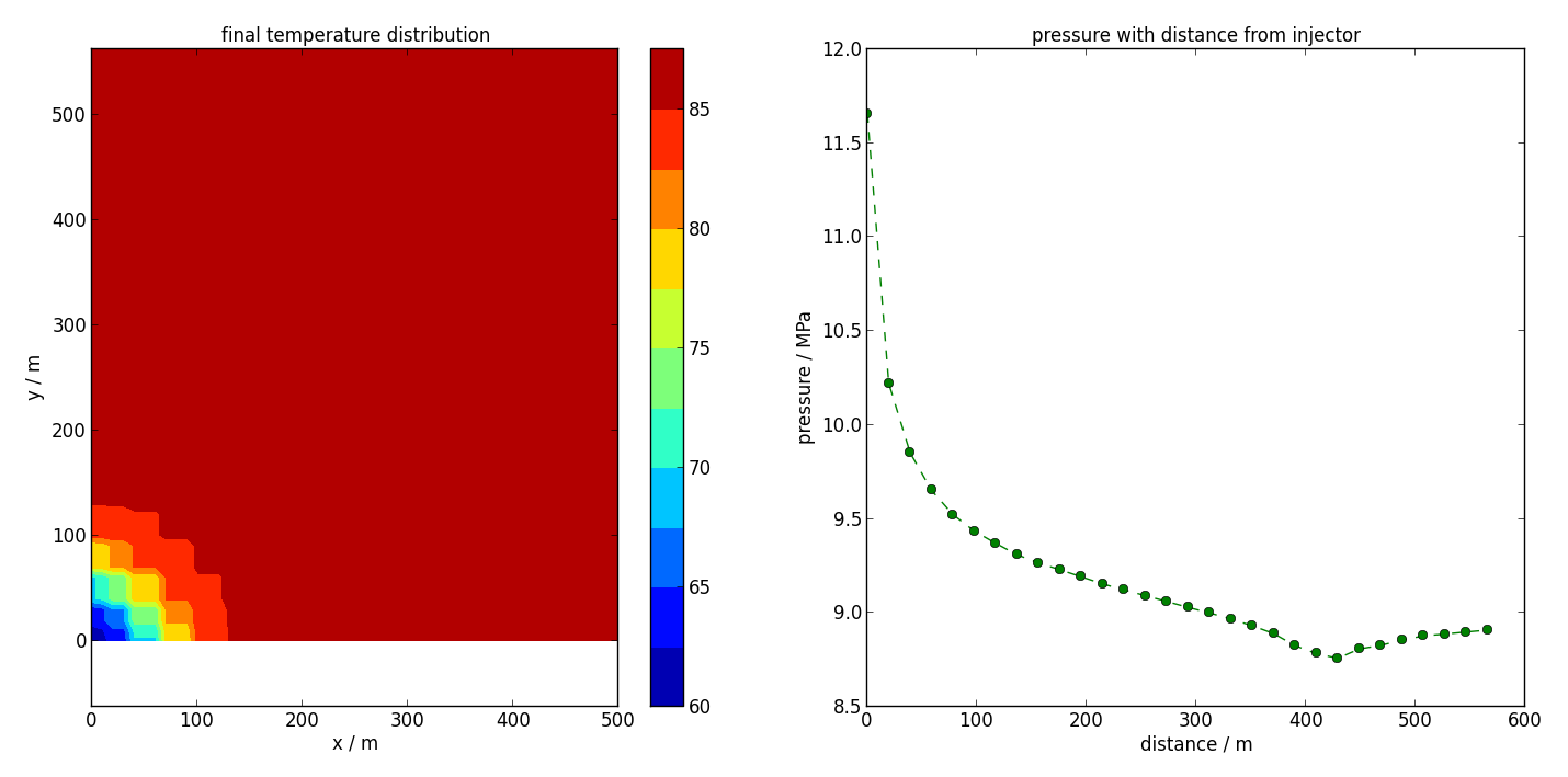
Left: Slice plot of final temperature distribution at z=-1000, as produced by slice_plot(). Right: Horizontal profile plot of pressure with distance from the injector, as produced by profile_plot().
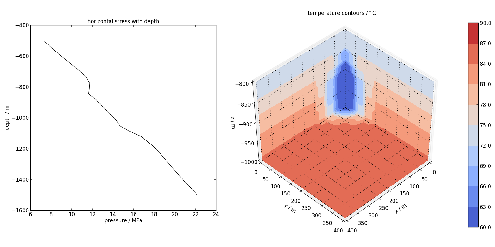
Left: Vertical profile plot of horizontal stress, as produced by profile_plot(). Right: Cutaway plot of temperature, as produced by cutaway_plot().

Time series plot of production flow rate, as produced by time_plot().
Multiprocessing and batch job submission
Having constructed and performed an FEHM simulation, often it is necessary to rerun the model for different parameter values. This could be for either calibration or parameter sensitivity purposes. In these situations, the models can be run as batches - with no requirement for information transfer between simulations, they can be run asynchronously in parallel.
Using Python’s multiprocessing module, we can generalise a script that creates, runs and postprocesses an FEHM simulation for one specific parameter set so as to distribute multiple simulations across a specified number of cores. As an example, we shall extend the first tutorial (Section 7.1).
Setting up a batch of simulations
First, import the multiprocessing module.
import multiprocessing
We will use indices to keep track of models. In this case, we will run the model four times with different parameters and so require indices 1 through 4, given by the range() command. Additionally, we will choose to distribute these jobs to two or our machine’s processors.
models = range(1,5)
processors = 2
Now we need to define the parameter sets for each of the four simulations. In this case, we are looking at two different permeabilities for the centre layer, and two different temperatures for the boundary condition at the base of the model. Each parameter set is a list, and all parameter sets are contained in a single list, i.e., a nested list structure. The formatting used below is simply a visual aide to keep track of simulations.
params = [
#[kmid,Tbase], # legend
[1.e-20,80], # 1
[1.e-20,120], # 2
[1.e-16,80], # 3
[1.e-16,120], # 4
]
Generalising to a function
In tutorial 1 (Section 7.1), we wrote a script to construct, run and post-process a simple FEHM simulation. As a first step, this script must be generalised as a callable function - this is relatively easy.
The corresponding function is defined by writing
def simulation(j,param):
and then indenting the rest of the script below this line (excluding import commands which should remain outside the function call). The name of the function is simulation and it receives two input arguments: j, an integer index indicating which model we are running, and param a list of parameters to be assigned within the function call. For example, in the case describe here param might contain [1.e-20,120], i.e., the second parameter set in the list of all parameter sets, params, defined in the previous section.
Parameters as function arguments
In tutorial 1, the parameters to be varied are defined explicitly in the script with the lines
kmid=1.e-20
dat.zone['ZMIN'].fix_temperature(80)
These lines need to be altered to reflect the general parameters supplied as the argument param. First, we will unpack the list param into separate variables by writing
kmid, Tbase = param
or equivalently
kmid=param[0]
Tbase=param[1]
Now, kmid is clearly defined, and we can simply delete the line reading
kmid=1.e=20
If left in, this would override the value of kmid passed as an argument to simulation.
In the case of Tbase, we need to replace the argument of fix_temperature`` so that it reads
dat.zone['ZMIN'].fix_temperature(Tbase)
Assigning the simulation a target directory
As we are performing four simulations, for the sake of tidiness, it makes sense that all files pertaining to a simulation should be placed in a separate simulation directory. This is necessary, as calling fehm.exe multiple times simultaneously in the same directory can lead to sharing issues.
Performing simulations in target directories is relatively simple with PyFEHM. The first step is to generate a different root label for each simulation, using the model index (passed to simulation as the argument j) to distinguish between each. We replace
root = 'tut1'
with
root = 'tut3_'+str(j)
which will yield root labels ‘tut3_1’, ‘tut3_2’, ‘tut3_3’ and ‘tut3_4’ for the four simulations.
Second, when the fdata object is created, we pass the root label to the input argument work_dir.
dat = fdata(work_dir=root)
This tells PyFEHM that all grid, input, incon and output files should be created in the new folder root inside the current work directory. Furthermore, the simulation itself is performed inside root and not the current directory.
Two additional changes are required in the post-processing section so that the correct files are targeted. These are
c=fcontour(root+'\\*.csv',latest=True)
and
c.slice_plot(save=root+'\\Tslice.png', cbar=True, levels=11, slice=['x',5], variable='T', method='linear', title='temperature / degC', xlabel='y / m', ylabel='z / m')
c.slice_plot(save=root+'\\Pslice.png', cbar=True, levels=np.linspace(4,6,9), slice=['x',5], variable='P', method='linear', title='pressure / MPa', xlabel='y / m', ylabel='z / m')
Assembling the processing pool and distributing the simulations
First, we write a simple function that, for a given model index, executes the simulation function (simulation) one time, passing it the correct input arguments. The name of this function will be execute() and its definition is given below.
def execute(j):
simulation(j,params[j-1])
Now there are simply two commands to submit the batch job. The first, multiprocessing.Pool assembles a pool of available processors that will be used to run simulations. As a simulation is complete, its processor is returned to the pool and is then available to run a new simulation. The second command maps the simulation function, as accessed through execution() with the set of models to be run models, defined in the first section. These two tasks are coded below
if __name__ == '__main__':
p=multiprocessing.Pool(processes = processors)
p.map(execute,models)
The if conditional preceding these commands is very important. Omitting this can lead to an infinite loop that spawns a new python process each time - this can rapidly overwhelm the system and is generally counterproductive.
Basic operation of the parallel batch script
When this modified script is executed, the following actions are executed
A pool of two available processors is assembled (multiprocessing.Pool).
Four indices (1,2,3, and 4) corresponding to four models (params[0], params[1], etc.) are submitted to the function execute. Because there are two available processors, execute proceeds with j=1 on the first and j=2 on the second.
execute passes both j and the parameter set params[j-1] to the function simulation(). This function
- Creates a new directory numbered by j.
- Creates a grid in that directory.
- Constructs and runs an FEHM model with the specific parameters in that directory.
- Post-processes output results in that directory.
When simulation and execution complete, the processor is returned to the pool. Model indices j=3 and j=4 are still waiting and will take these returned processors as they become available, executing step 3 themselves.
When all model indices have been input to and returned by execute, the batch simulation is complete.
Dynamic simulation monitoring
In some instances, the final simulation time for a model is specified as some arbitrarily large value. This is to ensure that the model doesn’t finish before the behaviour we are trying to model has. However, if we could observe the simulation as it proceeded, we could monitor for an arbitrary finish criterion and terminate the process when it is satisfied.
In this tutorial, we will demonstrate how to specify an arbitrary kill condition for a simulation - in this case, when the temperature at a particular node drops below a given value.
As in the previous tutorial, we will use as a basis the model developed in tutorial 1.
Defining a kill condition
First, the simulation time is doubled to 20 days.
dat.tf=20.
The kill condition is defined as a function with particular input and return conditions. The function must accept a single input, an fdata object, and return True or False depending on whether the condition has been satisfied.
This function is passed to the until argument in the run() method when the simulation is executed. In operation, the function is passed the fdata instance from which run() is called. PyFEHM monitors for output files containing information for a restart simulation that are periodically written by FEHM; these are parsed and the information made available at the nodal level. For example, nodal temperatures are available through the fnode.T attribute inside the function.
First define the function
def kill_condition(dat):
We want to set a kill condition when the node at position [7,7,9] has a temperature less than 50degC. First we need to locate that node
This node’s state attributes are updated at each time step during the simulation. Thus, all that is required is for us to test the kill condition
Now run the simulation with the modified run() method
dat.run(root+'_INPUT.dat',until=kill_condition)
This simulation now finishes after 5 time steps or approximately 13 days, instead of the 20 days specified as the end of the simulation.
Paraview visualisation
PyFEHM supports 3-D visualisation of model and output data in the software Paraview (www.paraview.org). Paraview must be installed ahead of time before For instance, the user can visualise various information on the model grid, e.g., material properties like permeability or porosity, zone information, or output data such as temperatures and pressures. Once loaded in Paraview, these data can be sliced, contoured and otherwise manipulated using Paraview’s built-in tools.
An instance of Paraview is initialised by calling the paraview() method, either from an fdata or fcontour object. Behind the scenes, PyFEHM formats and writes out grid, model and output data in the VTK format, and then subsequently loads these files into Paraview.
If a sequence of contour output data files are loaded in, then the user can optionally request two derived variables types. By passing the paraview() method diff=True, variable differences are created, e.g., the new variable T_diff will plot the change in temperature from its initial simulation value. By passing time_derivative=True, time derivatives for each variable will be calculated.
PyFEHM will assume that paraview.exe is available for command line execution. The user can ensure this is the case by including the folder containing the paraview executable in their PATH environment variable. Alternatively, the user can pass exe='/path/to/paraview.exe' directly to the paraview() method, or set this path in the config file.
Using the Paraview method
To get started, in tutorial1.py, uncomment the paraview command near the end of the script
Note that we have omitted the exe argument as it is expected that paraview.exe is available at the command line or otherwise defined in the config file. Because paraview is a method of fdata, it has access to all the zone, permeability, etc. information defined in that object. However, it has no knowledge of simulation output that is encapsulated in the fcontour object c defined in the previous command. Therefore, this object has to be explicitly passed to paraview via contour=c.
Running the script tutorial1.py, you should now see an instance of Paraview opened automatically (once the simulation has concluded). There is a short period of activity after Paraview has been opened that it is busy loading files, creating layers etc. - after this has finished you should see something like the figure below.
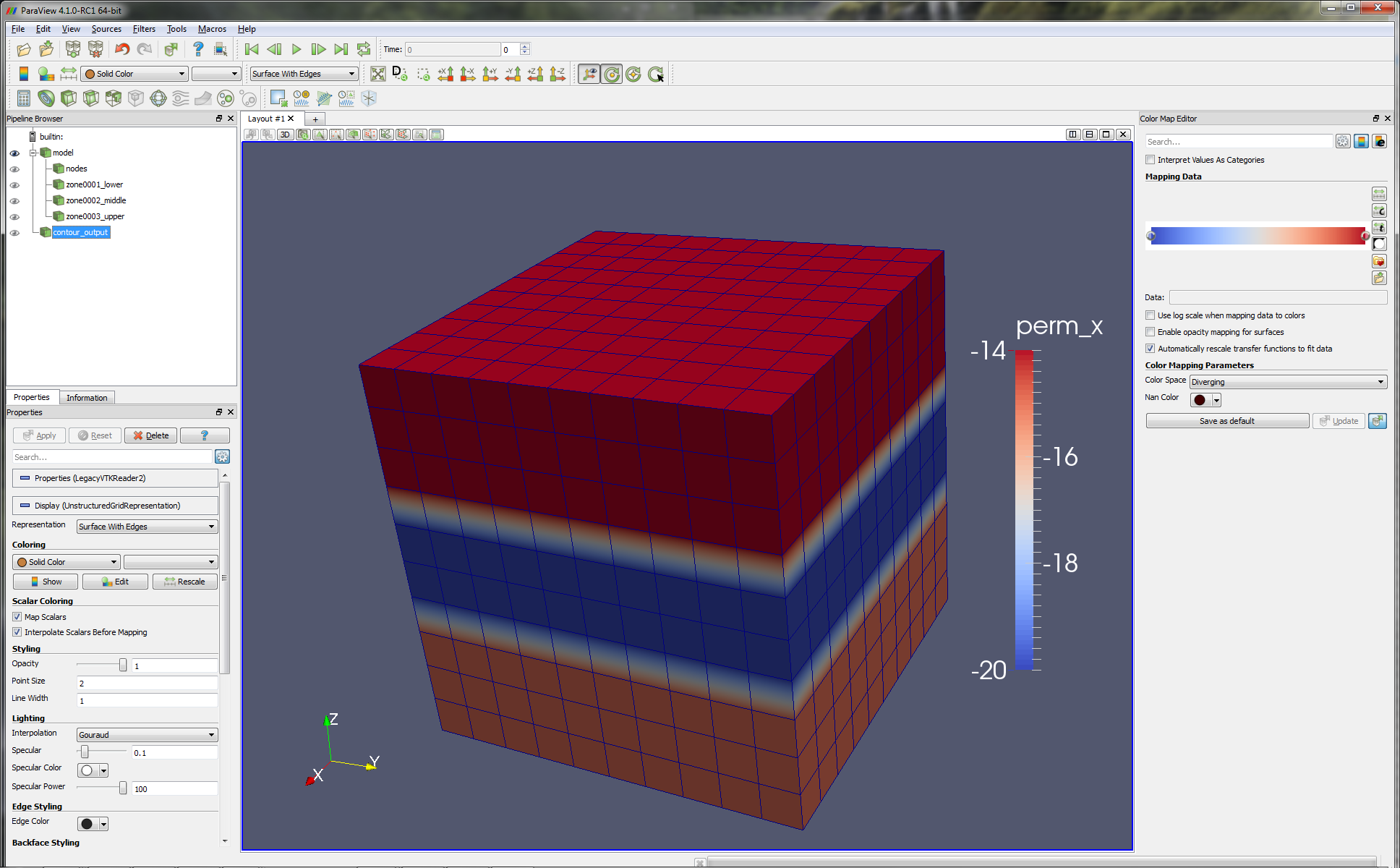
Model information
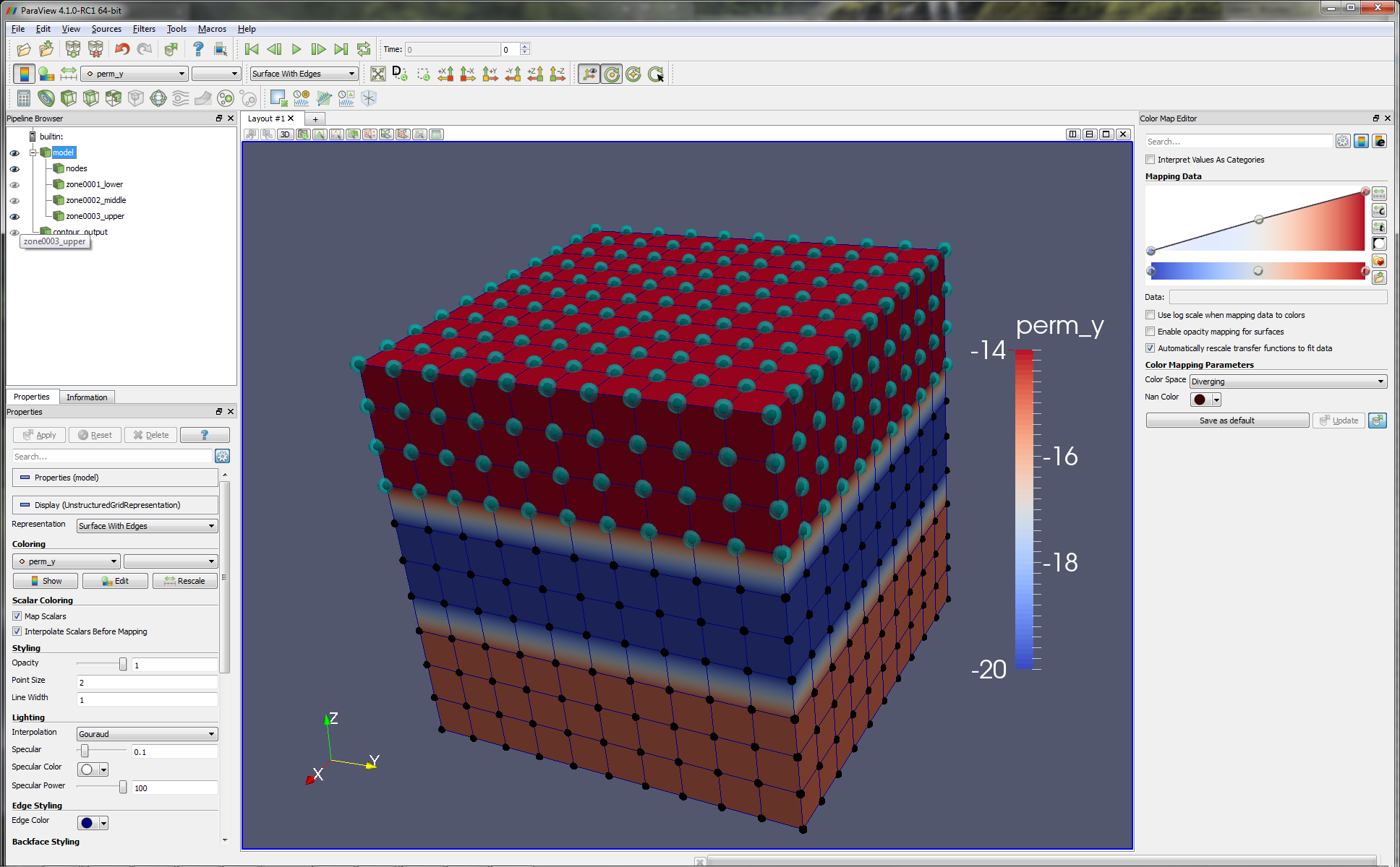
In the centre panel, a visualisation of the model is displayed, in this case contouring x permeability. A low permeability zone in the centre of the model, defined on the line
dat.zone[2].permeability=kmid
is evident, as well as the regular grid spacing, defined on the lines
x=np.linspace(0,10,11)
dat.grid.make(root+'_GRID.inp',x=x,y=x,z=x)
The top left panel contains a branching structure with members model and contour_output; these allow us to switch in and out various model information. For instance, with model selected use the drop-down menu to select zone_996_YMAX and note how the colouration changes to highlight the location of this zone.
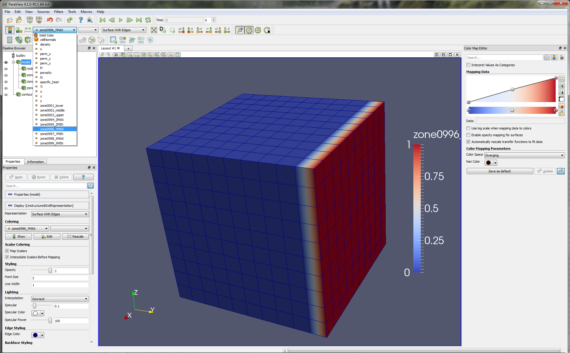
This type of visualisation can be a quick means of checking that zones a user has defined in a PyFEHM script (and are consequently represented in FEHM) actually correspond to the region of the model they have in mind. The paraview method does not require a simulation to have actually been executed before the model can be visualised; the method can be called on any ‘half-finished’ fdata object.
Within the model branch, you can choose to switch on node visualisation (by toggling the ‘eye’ symbol next to nodes) or just certain zones. By default, only user-defined zones are included here; however, visualisations for the boundary zones can be obtained by passing zones='all' when calling the paraview method.
Below we show the upper zone and nodes superimposed on a distribution of y permeability. In this way, it is evident that permeability is in some way linked to the definition of the upper zone (well obviously!) - in more complex simulations, this can be a good way to keep track of what material properties are being assigned where.
Contour output
The branch contour_output contains information from the contour object that we passed to paraview. This includes differenced or time derivative variables that may have been created by passing the relevant arguments to paraview. The model and contour_output branches are not mutually exclusive. For example, one could superimpose a zone or node visualisation from model on, say, temperature distributions in contour_output to get a sense of any correspondence between these items.
Turning off the model branch, and turning on contour_output (again using the ‘eye’ toggles), we are presented with a view of model pressures at the end of the simulation.
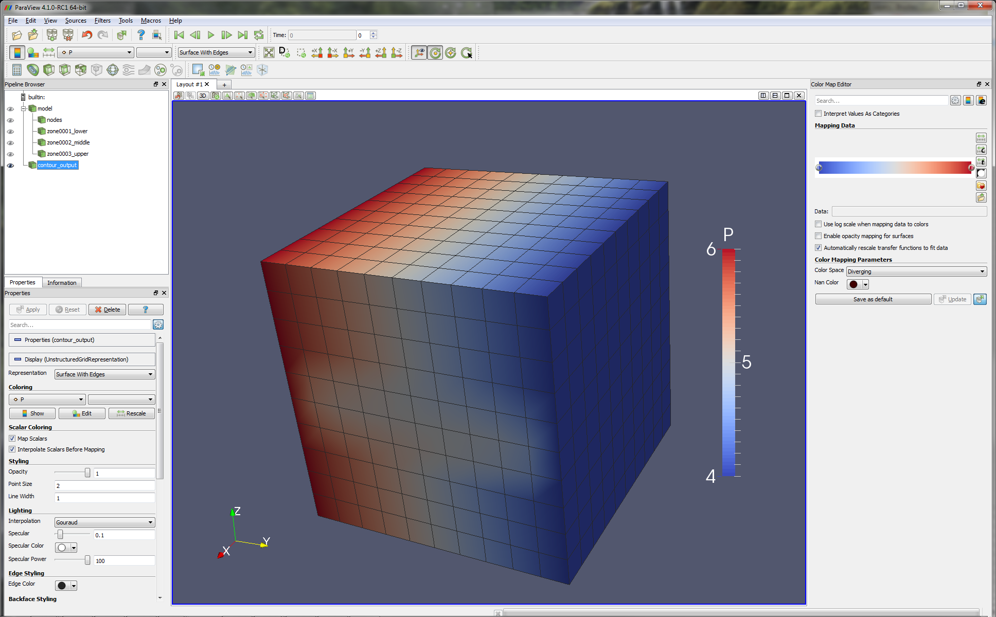
In this view, it is clear that the horizontal pressure gradient has been perturbed by the presence of the low permeability zone in the centre of the model.
We can look at other variables by selecting the model branch and using the same drop-down menu we earlier used to inspect material properties. Note that, in this menu, are the additional differenced and time derivative variables we requested to be defined.
Some additional Paraview tools
Here we briefly list several of Paraview’s useful visualisation features.
- Slices can be taken through a model to view material properties or output variables in the interior. Access this feature through Filters > Common > Clip or Slice.
- Isosurfaces can be defined that follow a specific zone: Filters > Common > Contour
- If multiple contour output files have been imported (corresponding to different output times), an animation can be played using the green animation buttons at the top of the screen.
- Save a visualisation via File > Save Screenshot.
For example, the figure below shows a vertical slice that clips away half the model. Grid lines are superimposed upon the solid section that remains, with the colouration corresponding to permeability. An isosurface has been constructed for the base of the reservoir zone and contours of pressure have been plotted on this isosurface.

Paraview script
Installation of PyFEHM provides access to the python script ‘fehm_paraview.py’. This script operates as an executable that accepts command line arguments and opens a Paraview visualisation of a particular FEHM simulation.
fehm_paraview.py resides in the /Scripts folder of your Python installation. If /Scripts is included in the PATH environment variable, and the default program for *.py files is Python (on Windows), then this script can be called as an executable.
In its simplest use, fehm_paraview.py can be called without arguments in any directory containing an ‘fehmn.files’ FEHM control file. For example, in running the script ‘tutorial1.py’, we created the subdirectory /tut1, which contains various simulation files, including ‘fehmn.files’ for that simulation. Navigate to this directory and at the command line execute
..\\pyfehm\\tutorials\\tut1>fehm_paraview.py
this will cause an instance of Paraview to be opened and initialised with all model, grid and contour output data. For more options on command line use of fehm_paraview.py, call this script with the --help argument
fehm_paraview.py --help
Diagnostic window
FEHM supplies a stream of information to the terminal when a simulation is running. For instance, time step size, number, elapsed time, mass and energy balances, residuals and some nodal information can all be reported. Often it may be useful to track and plot these information in time, particularly for long simulations with many time steps.
PyFEHM provides a diagnostic tool that both plots these data in real time and dumps the output information in column format to several auxiliary *.dgs files. Additional information is provided about ‘Largest N-R’ corrections that occur before time step cutbacks and provide and indication of which regions of the model FEHM is struggling to achieve convergence.
As for the previous section, the PyFEHM diagnostic tool will be demonstrated by modifying and running tutorial1.py. In this script, uncomment two lines before the run method
dat.tf=100.
dat.iter['machine_tolerance_TMCH']=-0.5e-5
The increased run time provides a better demo and the lower tolerance allows us to demonstrate time step cutbacks.
As in tutorial 1, the simulation is performed by calling the run method, but this time modified to pass diagnostic=True
dat.run(root+'_INPUT.dat',diagnostic=True)
As the simulation executes, a dialogue window will open with several empty ploting axes. These are populated as the simulation proceeds with information taken from the output stream.
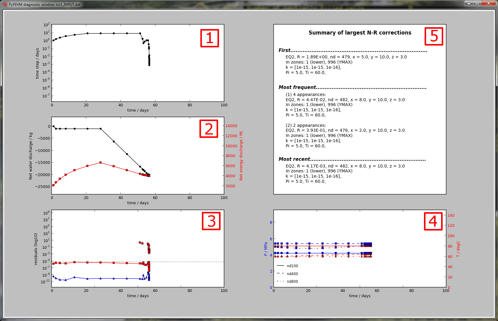
In the figure above, there are five boxes, numbered 1 through 5, containing different information. Each of these is explained below:
Time step size on a log-plot. Both the x and y axes will readjust dynamically depending on the range of data. If this curve starts trending down, it is an indication of time step cutbacks and convergence issues.
Net water (black) and energy (red) discharge. Appropriate y-scale is in the corresponding color.
Residuals on a log-scale for the each governing equation: mass (blue) and energy (red) balance, and, if running with the stress or CO2 modules, the static-force or CO2 balance (black). A dotted line shows the residual tolerance; if the residual exceeds this line, FEHM will cutback the time step to achieve better convergence.
Where Largest N-R corrections occur and the time-step is cutback, star symbols in the appropriate color are plotted, e.g., in the figure above, cutbacks occurred when the energy balance (red) residual exceeded the tolerance, hence red stars are plotted.
Node properties. FEHM outputs temperature, pressure and flow information to the screen for history nodes in dat.hist.nodelist. Up to the first four of these are plotted using different line styles (see legend). The first two variables defined in dat.hist.variablesare plotted on the two axes.
When Largest N-R corrections occur, it is useful to know what node they occurred at, what its material properties are, what zone it belongs in etc. This information is provided in Box 5, including (i) the first node to produce a Largest N-R cutback, (ii) the two most-frequent nodes that produced cutbacks, and (iii) the most-recent node to produce a cutback. The final two update as the simulation proceeds.
The diagnostic window has several interactive properties. It can be maximised/minimised, resized and moved around the screen. It can also be closed without interrupting the simulation. However, run method that produces the diagnostic window will not return until the window is closed; scripts will pause at the end of a simulation until the user intervenes.
Output files
In addition to visualising this information in the diagnostic window, PyFEHM writes the information in delimited format to three output files, named `*_convergence.dgs’, `*_NR.dgs’ and `*_node.dgs’. Alternatively, these output files can be produced by reading an FEHM ‘*.outp’ file (which contains the same terminal stream) using the process_output function.
- fdata.process_output(filename, input=None, grid=None, hide=False, silent=False, write=True)
Runs an FEHM *.outp file through the diagnostic tool. Writes output files containing simulation balance, convergence, time stepping information.
Parameters: - filename (str) – Path to the *.outp file.
- input (str) – Path to corresponding FEHM input file .
- grid (str) – Path to corresponding FEHM grid file.
- hide (bool) – Suppress diagnostic window (default False).
- silent (bool) – Suppress output to the screen (default False).
- write (bool) – Write output files (default True).
Diagnostic script
Similar to Paraview visualisation, a script is supplied on installation for command line execution of the diagnostic tool. This script should precede an FEHM executable call that would otherwise execute an FEHM simulation. For example, if the user has prepared a directory containing the control file ‘fehmn.files’, with directions to an FEHM input and grid file, then an FEHM simulation would be started by typing
tutorials\tut1>fehm.exe
at the command line (presuming that ‘fehm.exe’ is in the PATH). To perform the same simulation with a diagnostic window, simply precede the executable with ‘diagnose.py’
tutorials\tut1>diagnose.py fehm.exe
This will cause the simulation to be run through PyFEHM and a diagnostic window to be opened.
Additional instructions on making installed Python scripts available at the command line can be found in the previous section on Paraview visualisation.